2 Introduction to quantum mechanics
Quantum mechanics (QM) is the general theory to describe any microscopic phenomenon (until now), at low and high energies, for a few and infinitely many particles.
Its structure can be broken down into three main pieces that can be considered logically independent:
Classical mechanics \(F=ma\). As remarked in the third book by Landau (Landau and Lifshitz 1981), electrons, atoms, photons, and even subatomic particles are still described in terms of positions and velocities, following the algebraic relations of classical mechanics (non-relativistic or relativistic, depending). Somehow, this is the only way we have to build a measurable representation of nature. A physical system is thus defined by a set of degrees of freedom, which are quantified by vectors (non-relativistic, or 4-vectors relativistic) representing the canonical variables \(q,P\) of a Hamiltonian system. The Hamiltonian function \(H(q,P)\) generates the time evolution through the Hamilton equation (equivalent to the Euler-Lagrange equation and thus to the Newton equation).
Non-commuting variables. The canonical variables are non-commuting \([q,P]\neq 0\), and thus, on top of their vectorial character, they contain more information than purely classical ones. While transforming like classical vectors, quantum variables are not vectors representable with three real numbers, but rather matrices with complex entries. To preserve the Hamiltonian structure of classical mechanics, they require precise commutation relations, which are postulated to ensure consistency. More precisely, quantum variables are linear operators over a Hilbert space. Vectors of the Hilbert space represent the state of the system. A system composed by many subsystem has the structure of a tensor product of Hilbert spaces. Solving a quantum system means solving a multi-linear algebra problem.
Probabilistic interpretation, Born rule, and measurement postulate. Experiments on microscopic systems show random outcomes on single realizations. Quantum mechanics describes thus only the probability of finding a certain number in a measurement. This probability distribution is given by the state just before the measure, more precisely by its modulus square. After the measurement the state is randomly projected in an eigenstates of the measured quantity, where its eigenvalue is the measurement output. We postulate this is the theory, because none knows what happens during the measurement, but we know that is consistent with the experiments. While we cannot include the measurement in the theory, we can include its effect as a random projection.
Interestingly, it is very important to know well classical mechanics, and its Hamiltonian formulation in particular, for the correct formulation of the problem. All the equations are the same, and the basics rules for the approximations (small amplitude expansions, decoupling of time scales, adiabatic approximations...etc) are still valid (since they are very constrained by the algebric relations between the variables). The basics intuition about which degrees of freedom are most important, and who contributes more or less to the dynamics are still valid. A good knowledge of classical mechanics provides the basis to set our problem right!
Classical equations are not enough, and to solve them we need multi-linear algebra. Instead of looking for solving sets of ordinary differential equations (ODE) like in classical mechanics, we are left we an infinite linear system of differential equations. We loose complexity from the linearity, but we regain it from the infinite dimension of the Hilbert space! Here we need to introduce truncations to finite dimensions and linear algebra methods to actually solve the equations.
The result of our calculations will be probability amplitudes and expectation values, all to be interpreted in a probabilistic way. We will see that this probabilistic interpretation can also enter in the equation by using stochastic calculus and so-called Monte Carlo methods.
Notice that here we did not talk about wave equation and wave-particle duality. These concepts are still here, but hidden in the non-commutativity of the variables. Typically quantum theory is exposed starting indeed from the Schrödinger equation and with the De-Broglie wave-particle duality, but for our purposes is actually nicer to start from this other formulation. This way of thinking about quantum mechanics was originally introduced by Heisenberg (W. Heisenberg 1925, 1927; Born, Heisenberg, and Jordan 1926).
2.1 Short digression: Heisenberg’s matrix mechanics
While we often study QM from the wave-particle dualism and its Schrödinger formulation in terms of wave equation, it is worth noticing that the original Heisenberg’s formulation (+ Born and Jordan) had exactly this form, with a specific focus on the multi-linear algebra element. It is called matrix mechanics and, while Schrödinger formalism is quite handy for analytical solutions, matrix mechanics is essentially the most natural way to perform numerical computations. After 100 years, we go back to the origin!
Heisenberg took for granted that the microscopic world is still represented in term of canonical variables \(q,P, H(q,P)\) and Hamitonian equations \(\dot q = \partial_P H\), \(\dot P = -\partial_q H\). However he noticed that we never observe \(q,P\) of [e.g.] an atom or an electron, but rather the light emitted/scattered by these microscopic particles.
In particular he knew the Balmer-Lyman-Paschen-Brackett series of the lines of the hydrogen atom. These series say that the frequency of each emission/absorption line of the hydrogen atom is given by the formula
\[ \omega = \frac{R_Y}{\hbar}\left( \frac{1}{n^2} - \frac{1}{m^2} \right), \]
where \(n,m\in \mathbb{N}\), \(R_Y\) is the Rydberg constant and \(\hbar\) is the reduced Planck constant. Each observable frequency is determined by two integer numbers \(\omega_{nm}\), and it is thus natural to place it on a two-by-two table
\[ \begin{pmatrix} 0 & \omega_{01} & \omega_{02} & \omega_{03} & \ldots \\ \omega_{10} & 0 & \omega_{12} & \omega_{13} & \ldots \\ \omega_{20} & \omega_{21} & 0 & \omega_{23} & \ldots \\ \omega_{30} & \omega_{31} & \omega_{32} & 0 & \ldots \\ \vdots & \vdots & \vdots & \vdots & \ddots \\ \end{pmatrix} \]
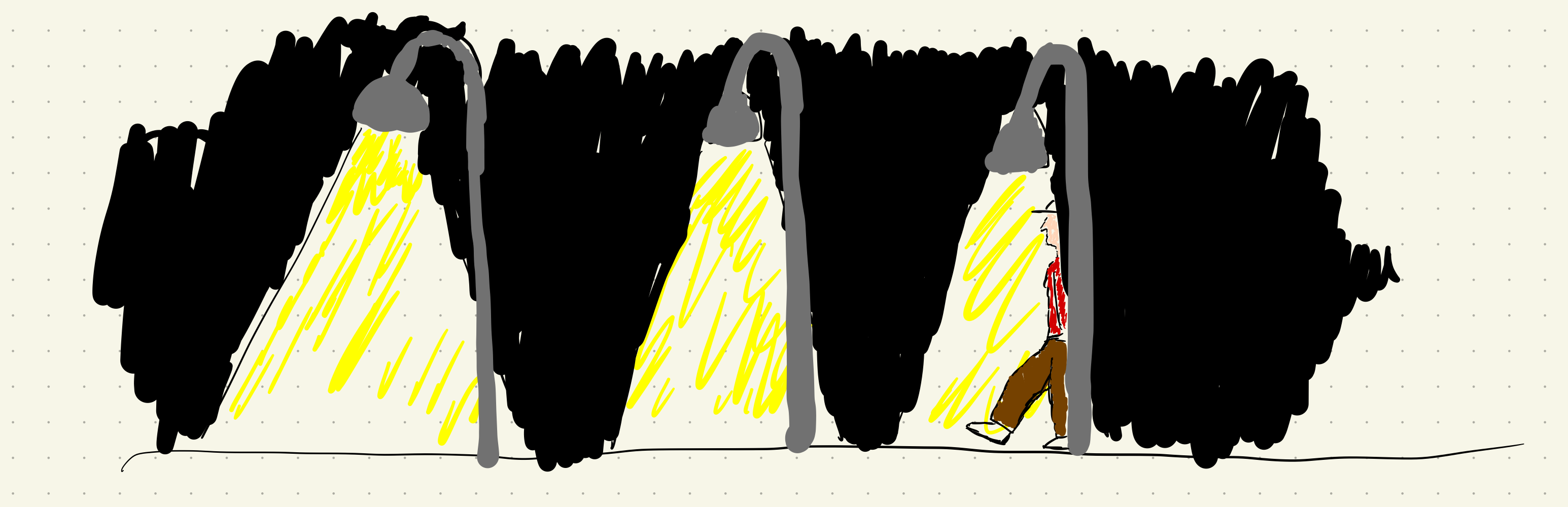
Each entry represents (according to Bohr) a jump between two stable orbits, or levels. However we only observe "transitions" between these orbits, and each single orbit is not observable even in principle. The position, velocity and everything measurable of a microscopic particle is then only defined during these jumps: it’s like watching someone at night under the street lights...(Werner Heisenberg 1958).
So Heisenberg postulates that all the quantities associated to a microscopic particle must be also given in two-by-two tables, where [e.g.] one can see the position or momentum of the hydrogen’s electron only during one of these transitions (after all we can just see the emitted light and its frequency). \[ q \longmapsto \begin{pmatrix} 0 & q_{01} & q_{02} & q_{03} & \ldots \\ q_{10} & 0 & q_{12} & q_{13} & \ldots \\ q_{20} & q_{21} & 0 & q_{23} & \ldots \\ q_{30} & q_{31} & q_{32} & 0 & \ldots \\ \vdots & \vdots & \vdots & \vdots & \ddots \\ \end{pmatrix} \]
These tables are not only a convenient way to visualize the observations, but they are the physical variables of the theory. We can interpret \(\lbrace{q_{nm}\rbrace}\) as a some sort of discretized version of the classical trajectory.
How do we use these tables to make theoretical predictions? A central problem for Heisenberg was how to sum and multiply these quantum variables, which are not numbers, but tables. The sum can be naturally taken as element-wise, but what about the multiplication? Heisenberg first noticed that the amplitude of emitted light also has a table \(\lbrace{a_{nm}\rbrace}\), and it must follow the time evolution \(a_{nm}\sim e^{-i\omega_{nm}t}\). Suppose we multiply two of these amplitudes, representing transitions sharing an equal level. In that case, we get another element that oscillates with a frequency of the table, \(a_{nk}a^{-i\omega_{nk}t}\,a_{km}e^{-i\omega_{km}t} = a_{nk}a_{km}e^{-i\omega_{nm} t}\), because \(\omega_{nk} + \omega_{km} = \omega_n - \omega_k + \omega_k - \omega_m = \omega_{nm}\) by definition. But the same is true if we sum over all possible \(k\). Here it is not so easy to understand how Heisenberg went on (perhaps who know german very well could read Refs. (W. Heisenberg 1925, 1927; Born, Heisenberg, and Jordan 1926) and figure it out directly at the source), but, under the suggestion of Born and Jordan, they recognized that multiplication between physical variable represented as tables can be obtained using the matrix multiplication rule (which at the time was mostly unknown), \(q_{nm}^2 = \sum_k q_{nk}q_{km}\).
Interestingly, they immediately noticed that this implies the non-commutativity \([\hat{q},\hat{P}]\neq 0\), which in principle seems not to be fixed (from here on we use that hat-notation \(\hat{q}\) to indicate the quantum variable as a table, or in a more modern language, operator). However, they noticed that for consistency between the "oscillator" character of the tables (each element \(a_{nm}\) must evolve as an harmonic oscillator at the given frequency \(\omega_{nm}\)), and the equation of the Hamiltonian mechanics there must be a precise commutation relation between \(q,P\). Let’s indeed consider that, as harmonically oscillating variables, each table element must follow
\[ \partial_t q_{nm} = -i\omega_{nm}q_{nm} = -\frac{i}{\hbar} [H, q]_{nm} \qquad \partial_t P_{nm} = -i\omega_{nm}P_{nm} = -\frac{i}{\hbar} [H, P]_{nm}. \]
The use of the commutator and the Hamiltonian function here is justified by Bohr’s theory, where the frequencies are given by energy levels \(\omega_{nm} = (E_n - E_m)/\hbar\), and the energy is given by the Hamiltonian, which must be a diagonal table. Assuming \(H = P^2/(2m) + V(q)\), if we compare these equations with Hamilton’s
\[ \partial_t \hat{q} = \hat{P}/m \qquad \partial_t\hat{P} = - \partial_{\hat{q}}V(\hat{q}), \]
we have that \[ P_{nm} = -im \,\omega_{nm}q_{nm} \qquad [\partial_qV(q)]_{nm} = \frac{i}{\hbar} [H, P]_{nm}. \]
Using \(V(q) = - q\) we have that
\[ [\hat{q},\hat{P}] = i\hbar \hat{\mathbb{1}} . \]
Interestingly, the consistency between the existence of Bohr’s levels, the oscillating origin of microscopic physical variables and Hamilton’s equations implies a linear algebra structure that must be defined on an infinite dimensional vector space. A hint for this surprising consequence immediately comes by noticing
\[ {\mathrm Tr}(\hat{q}\hat{P}-\hat{P}\hat{q}) = {\mathrm Tr}(\hat{q}\hat{P}) - {\mathrm Tr}(\hat{P}\hat{q}) = {\mathrm Tr}(\hat{q}\hat{P}) - {\mathrm Tr}(\hat{q}\hat{P}) = 0 \neq i\hbar {\mathrm Tr}(\hat{\mathbb{1}}) = \infty. \]
In any finite-dimensional space, this commutator cannot be proportional to the identity!
2.2 Exercise: the harmonic oscillator
Let’s consider the example reported in the excellent book of Max Born (Born, Blin-Stoyle, and Radcliffe 1989): the harmonic oscillator.
\[ \hat{H} = \frac{\hat{P}^2}{2m} + \frac{m \omega^2}{2}\hat{q}^2, \]
whose Hamilton equations are given by
\[ \partial_t \hat{P} = - m \omega^2 \hat{q} \qquad \partial_t \hat{q} = \frac{\hat{P}}{m}, \]
giving
\[ \partial_t^2 \hat{q} = - \omega^2 \hat{q}. \]
Following Heisenberg, this must be true for each element of the corresponding quantum table [matrix, or operator], which, at the same time, must follow an oscillatory dynamics
\[ q_{nm}(t) = q_{nm}(0) e^{-i\omega_{nm} t }. \]
Putting them together we find that \((\omega_{nm}^2 - \omega) q_{nm} = 0\), implying that \(\omega_{nm} = \pm \omega\) and necessarily
\[ q_{nm}(0) = 0 ~~~ {\mathrm if~~~}m\neq n+1 \qquad q_{nm}(0)\neq 0 ~~~{\mathrm if}~~~m=n+1. \]
We thus find the structure \[ \hat{q} = \begin{pmatrix} 0 & q_{01} & 0 & 0 & \ldots \\ q_{10} & 0 & q_{12} & 0 & \ldots \\ 0 & q_{21} & 0 & q_{23} & \ldots \\ 0 & 0 & q_{32} & 0 & \ldots \\ \vdots & \vdots & \vdots & \vdots & \ddots \\ \end{pmatrix} \]
and from \(P_{nm} = i m \omega_{nm} q_{nm}\),
\[ \hat{P} = im\omega \begin{pmatrix} 0 & -q_{01} & 0 & 0 & \ldots \\ q_{10} & 0 & -q_{12} & 0 & \ldots \\ 0 & q_{21} & 0 & -q_{23} & \ldots \\ 0 & 0 & q_{32} & 0 & \ldots \\ \vdots & \vdots & \vdots & \vdots & \ddots \\ \end{pmatrix} \]
Using the commutation relation \([\hat{q}, \hat{P}] = i\hbar \hat{\mathbb{1}}\) we have that
\[\begin{align} & -2im\omega \begin{pmatrix} q_{01}q_{10} & 0 & 0 & 0 & \ldots \\ 0 & q_{12}q_{21} - q_{01}q_{10} & 0 & 0 & \ldots \\ 0 & 0 & q_{23}q_{32} - q_{12}q_{21} & 0 & \ldots \\ 0 & 0 & 0 & q_{34}q_{43} - q_{23}q_{32} & \ldots \\ \vdots & \vdots & \vdots & \vdots & \ddots \\ \end{pmatrix} \\ &= i\hbar \begin{pmatrix} 1 & 0 & 0 & 0 & \ldots \\ 0 & 1 & 0 & 0 & \ldots \\ 0 & 0 & 1 & 0 & \ldots \\ 0 & 0 & 0 & 1 & \ldots \\ \vdots & \vdots & \vdots & \vdots & \ddots \\ \end{pmatrix} \end{align}\]
from which we derive the recurrence formula
\[ q_{n\,n+1}q_{n+1\,n} = |q_{n\,n+1}|^2 = (n+1)\frac{\hbar}{2m \omega}, \]
and
\[ H_{nn} = m\omega^2\left( |q_{n\,n+1}|^2 + |q_{n\,n-1}|^2 \right) = \frac{\hbar \omega}{2}\left(2n + 1\right). \]
2.3 Being practical
After Dirac and Von Neumann we now know that there is more in quantum mechanics than "tables", commutator and oscillating elements. Indeed, having an Hilbert space for the linear operators directly implies the existence of states of the Hilbert space that constitute the domains of such operators. Moreover the linear algebra structure is also not sufficient, since for many particles we need a tensor product, and so we rather deal with multi-linear algebra. But the core of Heisenberg’s matrix mechanics and his perspective on quantum theory are still very central, as it will be clear in the rest of the course. What we do is in practice very similar in its logic:
find all the degrees of freedom describing your problem as you would do in classical physics [e.g. define particle positions \(x_1,x_2,x_3\ldots\), or any generalized coordinate system \(q\), or voltages and magnetic flux in circuit \(V,\Phi\), or even fields like \(\mathbf{E}(\mathbf{r}), \mathbf{B}(\mathbf{r})\)...].
use the equation of motions from classical mechanics to derive a Lagrangian and then an Hamiltonian with canonical variables generically labelled as \(q,P\). Here you could eventually employ approximations based on energy-time scales considerations (small amplitude oscillations, adiabatic elimination of fast variables etc...). This last sentence is not rigorous, but most of the time it works in the spirit of this quantum to classical relation.
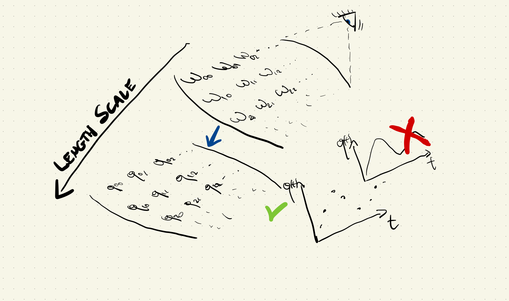
impose the canonical commutation relations \([\hat{q}, \hat{P}] = i\hbar\). Now the canonical variables (whatever they are) are interpreted as linear operators on an infinite dimensional Hilbert space \(\mathcal{H}\) (Heisenberg’s tables). This procedure preserves the algebraic relations between canonical variables given by Hamiltonian mechanics and, as Dirac showed, is equivalent to replacing Poisson brackets with commutator.
find a good basis \(\lbrace{|n \rangle \rbrace}\) for \(\mathcal{H}\) and represent all the operators as infinite matrices by computing their matrix elements \(\langle{n | \hat{A}|m\rangle}\) (\(\hat{A}\) is an arbitrary operator of the considered problem).
truncate the Hilbert space and make the matrices finite.
finite dimensional matrices are typical objects well suitable for digital processors, so make numerics on a computer.
interpret the results probabilistically using the Born rule.