13  Resonance Fluorescence and the Mollow Triplet

When a resonant laser drives a two‑level atom strongly, its resonance‑fluorescence spectrum splits into three Lorentzian peaks: a central line at the laser frequency and two symmetric sidebands. Predicted by B.R. Mollow in 1969 (Mollow (1969)) and first observed soon after, this Mollow triplet is a hallmark of light–matter interaction in the strong‑drive (dressed‑state) regime.

13.1 Physical picture

Consider a two‑level atom with energy separation \(\omega_0\) driven by a coherent laser at frequency \(\omega_L\).

\[ H = \frac{\omega_0}{2}\,\hat{\sigma}_z + \frac{\Omega}{2}\,(\hat{\sigma}_+e^{-i\omega_L t} + \hat{\sigma}_-e^{+i\omega_L t}). \]

Transforming to the laser rotating frame with \(U(t)=\exp [-i \tfrac{\omega_L t}{2}\hat{\sigma}_z]\) removes the explicit time dependence and shifts the zero of energy, yielding the textbook Hamiltonian used below

\[ H = \frac{\Delta}{2}\,\hat{\sigma}_z + \frac{\Omega}{2}\,(\hat{\sigma}_+ + \hat{\sigma}_-), \]

with detuning \(\Delta = \omega_0 - \omega_L\) and on‑resonance Rabi frequency \(\Omega = \mu E_0/\hbar\). This semiclassical model, combined with a Lindblad dissipator for spontaneous emission at rate \(\gamma\), fully captures the triplet.

13.2 Analytic spectrum

In order to analyse the properties of the emitted light, we can compute the power spectrum of the scattered photons, defined as the Fourier transform of the correlation function \(\langle \hat{E}^{(-)}(t) \hat{E}^{(+)}(0) \rangle\), where \(\hat{E}^{(-)}\) and \(\hat{E}^{(+)}\) are the negative and positive frequency parts of the electric field operator. In the rotating frame, these operators are related to the atom’s raising and lowering operators \(\hat{\sigma}_+\) and \(\hat{\sigma}_-\) as (Walls and Milburn 2008)

\[ \hat{E}^{(-)}(t) \propto \hat{\sigma}_+(t) \quad \text{and} \quad \hat{E}^{(+)}(t) \propto \hat{\sigma}_-(t) \, . \]

The power spectrum is then given by

\[ S(\omega) = \int_{-\infty}^{\infty} e^{i\omega t} \langle \hat{E}^{(-)}(t) \hat{E}^{(+)}(0) \rangle dt \, . \tag{13.1}\]

Treating spontaneous emission at rate \(\gamma\) with a Lindblad term \(\hat{L} = \sqrt{\gamma},\hat{\sigma}_-\), the power spectrum of scattered photons is (Walls and Milburn 2008)

\[ S(\omega) \propto \frac{\tfrac{\gamma}{2}}{(\omega-\omega_L)^2 + (\tfrac{\gamma}{2})^2} + \frac{3\gamma/8}{(\omega-\omega_L-\Omega_R)^2 + (3\gamma/4)^2} + \frac{3\gamma/8}{(\omega-\omega_L+\Omega_R)^2 + (3\gamma/4)^2}. \]

with a central peak at \(\omega_L\) and two sidebands at \(\omega_L \pm \Omega_R\), where \(\Omega_R = \sqrt{\Delta^2 + \Omega^2}\) is the Rabi frequency in the rotating frame.

13.3 Numerical spectrum in QuTiP

Below is a minimal QuTiP script that reproduces the triplet for a resonantly driven atom (\(\Delta = 0\)). The code computes the emission spectrum \(S(\omega)\) in Equation 13.1 by using the spectrum function to compute the Fourier transform of the correlation function of the emission operators.

import numpy as np
import matplotlib.pyplot as plt
from qutip import *

gamma = 1.0          # spontaneous emission rate
Omega = 5.0 * gamma   # Rabi frequency (drive strength)
Delta = 0.0           # laser detuning

sm = sigmam()
sp = sigmap()
sz = sigmaz()

H = 0.5 * Delta * sz + 0.5 * Omega * (sp + sm)
c_ops = [np.sqrt(gamma) * sm]

rho_ss = steadystate(H, c_ops)

wlist = np.linspace(-10 * gamma, 10 * gamma, 2000)
S = spectrum(H, wlist, c_ops, sp, sm)
S /= np.max(S)

plt.plot(wlist / gamma, S)
plt.xlabel(r"$(\omega - \omega_L)/\gamma$")
plt.ylabel(r"$S(\omega)$ (arb. units)")
plt.title("Mollow triplet")
plt.xlim(-10, 10)

# Show in Quarto
plt.savefig("_tmp_fig.svg")
plt.close()
SVG("_tmp_fig.svg")

Running the code with \(\Omega = 5,\gamma\) reproduces the canonical spectrum: a narrow central line and two broader sidebands at \(\pm\Omega\).

13.4 Photon statistics and antibunching

Given the emission spectrum, we may ask if the emitted light is classical or quantum. The answer can be found in the photon statistics of the resonance fluorescence, which can be probed by measuring the second‑order correlation function

\[ g^{(2)}(\tau) \;=\; \frac{\langle\hat{E}^{(-)}(0)\,\hat{E}^{(-)}(\tau)\,\hat{E}^{(+)}(\tau)\,\hat{E}^{(+)}(0)\rangle}{\langle\hat{E}^{(-)}\hat{E}^{(+)}\rangle^{2}} \;\propto\; \frac{\langle\sigma^\dagger(0)\,\sigma^\dagger(\tau)\,\sigma^-(\tau)\,\sigma^-(0)\rangle}{\langle\sigma^\dagger\sigma^-\rangle^{2}} . \tag{13.2}\]

where \(\hat{E}^{(+)}\) and \(\hat{E}^{(-)}\) are the positive and negative frequency parts of the electric field operator, and \(\sigma^\dagger\), \(\sigma^-\) are the raising and lowering operators of the two‑level atom. The quantity \(g^{(2)}(\tau)\) measures the probability of detecting one photon at time \(0\) and another at time \(\tau\), normalised by the square of the average number of photons emitted.

For classical light \(g^{(2)}(0) \ge 1\) (photon bunching), whereas a single quantum emitter produces antibunching with \(g^{(2)}(0)=0\): once a photon is emitted, the atom is in its ground state and cannot emit another immediately, so the probability of detecting two photons with zero delay vanishes.

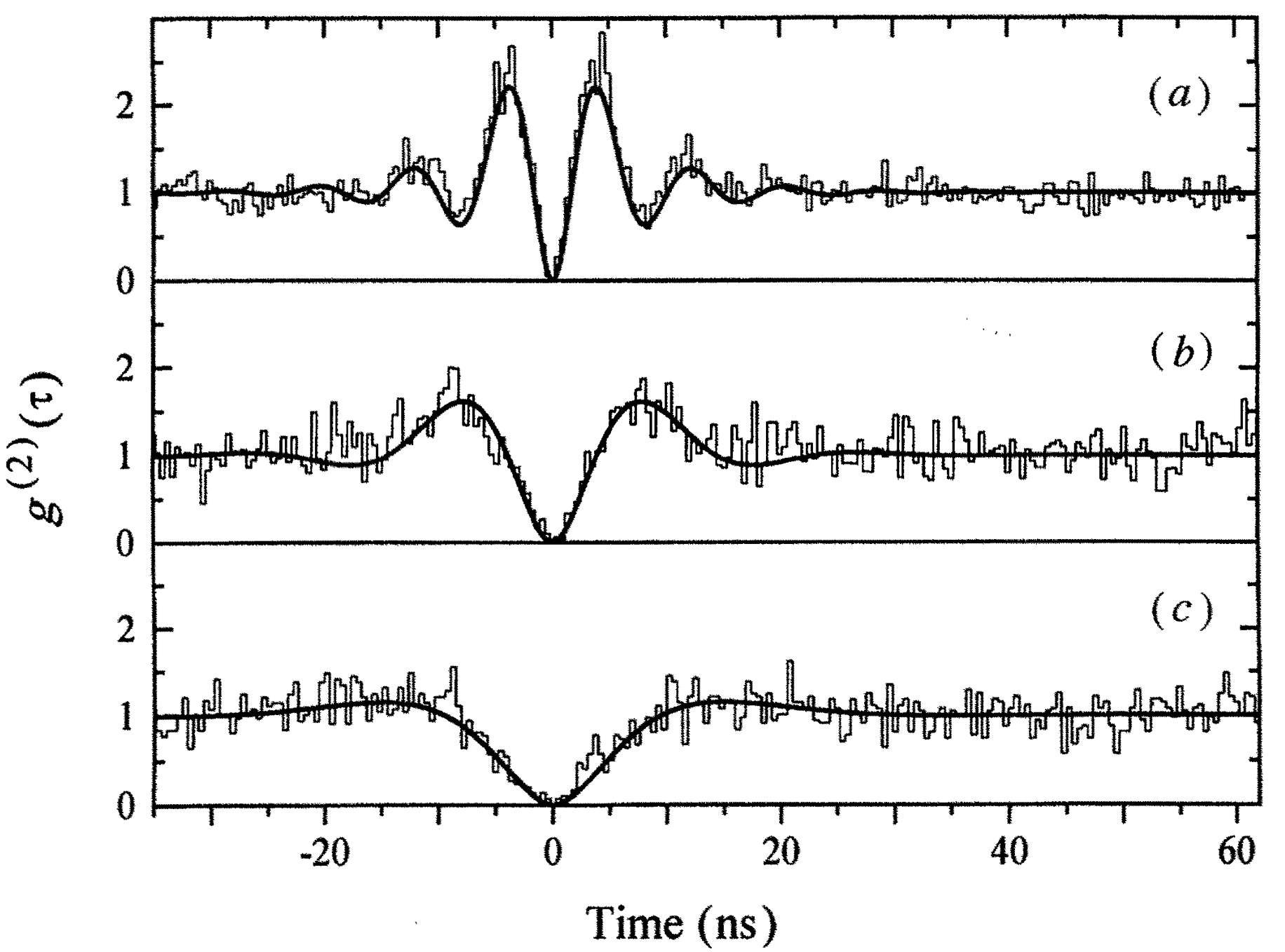
Under strong driving \(g^{(2)}(\tau)\) also displays damped Rabi oscillations at \(\Omega_R\)—a direct time‑domain analogue of the sidebands.

13.4.1 QuTiP example

tau_list = np.linspace(0, 10 / gamma, 400)  # time delays

rho_ss = steadystate(H, c_ops)

corr = correlation_3op_1t(H, None, tau_list, c_ops, sp, sp*sm, sm)

n_ss = expect(sp * sm, rho_ss) # steady‑state population
g2 = np.real(corr) / (n_ss ** 2) # normalized

plt.plot(tau_list, g2)
plt.xlabel(r"$\tau$")
plt.ylabel(r"$g^{(2)}(\tau)$")
plt.title("Photon antibunching and Rabi oscillations")
plt.ylim(0, None)

# Show in Quarto
plt.savefig("_tmp_fig.svg")
plt.close()
SVG("_tmp_fig.svg")

The plot shows \(g^{(2)}(0) \approx 0\) (perfect antibunching in the ideal model). As \(\tau\) increases the function overshoots above 1 and undergoes damped oscillations at the Rabi frequency before relaxing to the Poissonian value \(g^{(2)}(\infty)=1\).

The second order correlation function of the fluorescent light form a single mercury ion in a trap versus delay time \(\tau\). The antibunching at \(\tau=0\) is clearly visible, as well as the Rabi oscillations at longer delays. Figure taken from (Walther 1998).

13.5 Discussion

• Antibunching ⇒ unambiguously indicates a single quantum emitter or sub‑Poissonian light.
• Rabi oscillations in \(g^{(2)}\) ⇒ time‑domain fingerprint of the dressed‑state splitting that generates the Mollow sidebands.
• Technological relevance ⇒ Resonance‑fluorescence photons combine single‑photon purity (antibunching) with high brightness and tunable frequency via the drive laser.

Mollow, B. R. 1969. “Power Spectrum of Light Scattered by Two-Level Systems.” Phys. Rev. 188 (December): 1969–75. https://doi.org/10.1103/PhysRev.188.1969.

Walls, DF, and Gerard J Milburn. 2008. Quantum Optics. Springer Berlin Heidelberg. https://doi.org/10.1007/978-3-540-28574-8.

Walther, H. 1998. “Single atom experiments in cavities and traps.” Proceedings of the Royal Society of London. Series A: Mathematical, Physical and Engineering Sciences 454 (1969): 431–45. https://doi.org/10.1098/rspa.1998.0169.